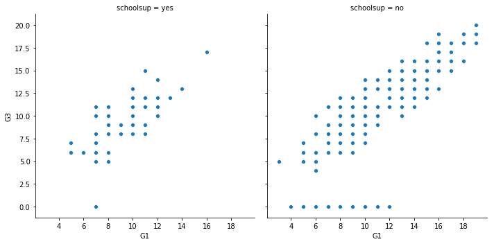
Changing the style of scatter plot points
Let's continue exploring Seaborn's mpg dataset by looking at the relationship between how fast a car can accelerate ("acceleration") and its fuel efficiency ("mpg"). Do these properties vary by country of origin ("origin")?
Note that the "acceleration" variable is the time to accelerate from 0 to 60 miles per hour, in seconds. Higher values indicate slower acceleration.
# Import Matplotlib and Seaborn
import matplotlib.pyplot as plt
import seaborn as sns
import pandas as pd

url = 'https://assets.datacamp.com/production/repositories/3996/datasets/e0b285b89bdbfbbe8d81123e64727ff150d544e0/mpg.csv'
mpg = pd.read_csv(url)
print(mpg)
mpg cylinders displacement horsepower weight acceleration \
0 18.0 8 307.0 130.0 3504 12.0
1 15.0 8 350.0 165.0 3693 11.5
2 18.0 8 318.0 150.0 3436 11.0
3 16.0 8 304.0 150.0 3433 12.0
4 17.0 8 302.0 140.0 3449 10.5
5 15.0 8 429.0 198.0 4341 10.0
6 14.0 8 454.0 220.0 4354 9.0
7 14.0 8 440.0 215.0 4312 8.5
8 14.0 8 455.0 225.0 4425 10.0
9 15.0 8 390.0 190.0 3850 8.5
10 15.0 8 383.0 170.0 3563 10.0
11 14.0 8 340.0 160.0 3609 8.0
12 15.0 8 400.0 150.0 3761 9.5
13 14.0 8 455.0 225.0 3086 10.0
14 24.0 4 113.0 95.0 2372 15.0
15 22.0 6 198.0 95.0 2833 15.5
16 18.0 6 199.0 97.0 2774 15.5
17 21.0 6 200.0 85.0 2587 16.0
18 27.0 4 97.0 88.0 2130 14.5
19 26.0 4 97.0 46.0 1835 20.5
20 25.0 4 110.0 87.0 2672 17.5
21 24.0 4 107.0 90.0 2430 14.5
22 25.0 4 104.0 95.0 2375 17.5
23 26.0 4 121.0 113.0 2234 12.5
24 21.0 6 199.0 90.0 2648 15.0
25 10.0 8 360.0 215.0 4615 14.0
26 10.0 8 307.0 200.0 4376 15.0
27 11.0 8 318.0 210.0 4382 13.5
28 9.0 8 304.0 193.0 4732 18.5
29 27.0 4 97.0 88.0 2130 14.5
.. ... ... ... ... ... ...
368 27.0 4 112.0 88.0 2640 18.6
369 34.0 4 112.0 88.0 2395 18.0
370 31.0 4 112.0 85.0 2575 16.2
371 29.0 4 135.0 84.0 2525 16.0
372 27.0 4 151.0 90.0 2735 18.0
373 24.0 4 140.0 92.0 2865 16.4
374 23.0 4 151.0 NaN 3035 20.5
375 36.0 4 105.0 74.0 1980 15.3
376 37.0 4 91.0 68.0 2025 18.2
377 31.0 4 91.0 68.0 1970 17.6
378 38.0 4 105.0 63.0 2125 14.7
379 36.0 4 98.0 70.0 2125 17.3
380 36.0 4 120.0 88.0 2160 14.5
381 36.0 4 107.0 75.0 2205 14.5
382 34.0 4 108.0 70.0 2245 16.9
383 38.0 4 91.0 67.0 1965 15.0
384 32.0 4 91.0 67.0 1965 15.7
385 38.0 4 91.0 67.0 1995 16.2
386 25.0 6 181.0 110.0 2945 16.4
387 38.0 6 262.0 85.0 3015 17.0
388 26.0 4 156.0 92.0 2585 14.5
389 22.0 6 232.0 112.0 2835 14.7
390 32.0 4 144.0 96.0 2665 13.9
391 36.0 4 135.0 84.0 2370 13.0
392 27.0 4 151.0 90.0 2950 17.3
393 27.0 4 140.0 86.0 2790 15.6
394 44.0 4 97.0 52.0 2130 24.6
395 32.0 4 135.0 84.0 2295 11.6
396 28.0 4 120.0 79.0 2625 18.6
397 31.0 4 119.0 82.0 2720 19.4
model_year origin name
0 70 usa chevrolet chevelle malibu
1 70 usa buick skylark 320
2 70 usa plymouth satellite
3 70 usa amc rebel sst
4 70 usa ford torino
5 70 usa ford galaxie 500
6 70 usa chevrolet impala
7 70 usa plymouth fury iii
8 70 usa pontiac catalina
9 70 usa amc ambassador dpl
10 70 usa dodge challenger se
11 70 usa plymouth 'cuda 340
12 70 usa chevrolet monte carlo
13 70 usa buick estate wagon (sw)
14 70 japan toyota corona mark ii
15 70 usa plymouth duster
16 70 usa amc hornet
17 70 usa ford maverick
18 70 japan datsun pl510
19 70 europe volkswagen 1131 deluxe sedan
20 70 europe peugeot 504
21 70 europe audi 100 ls
22 70 europe saab 99e
23 70 europe bmw 2002
24 70 usa amc gremlin
25 70 usa ford f250
26 70 usa chevy c20
27 70 usa dodge d200
28 70 usa hi 1200d
29 71 japan datsun pl510
.. ... ... ...
368 82 usa chevrolet cavalier wagon
369 82 usa chevrolet cavalier 2-door
370 82 usa pontiac j2000 se hatchback
371 82 usa dodge aries se
372 82 usa pontiac phoenix
373 82 usa ford fairmont futura
374 82 usa amc concord dl
375 82 europe volkswagen rabbit l
376 82 japan mazda glc custom l
377 82 japan mazda glc custom
378 82 usa plymouth horizon miser
379 82 usa mercury lynx l
380 82 japan nissan stanza xe
381 82 japan honda accord
382 82 japan toyota corolla
383 82 japan honda civic
384 82 japan honda civic (auto)
385 82 japan datsun 310 gx
386 82 usa buick century limited
387 82 usa oldsmobile cutlass ciera (diesel)
388 82 usa chrysler lebaron medallion
389 82 usa ford granada l
390 82 japan toyota celica gt
391 82 usa dodge charger 2.2
392 82 usa chevrolet camaro
393 82 usa ford mustang gl
394 82 europe vw pickup
395 82 usa dodge rampage
396 82 usa ford ranger
397 82 usa chevy s-10
[398 rows x 9 columns]# Import Matplotlib and Seaborn
import matplotlib.pyplot as plt
import seaborn as sns
# Create a scatter plot of acceleration vs. mpg
sns.relplot(x='acceleration', y='mpg',
data=mpg,
kind='scatter',
style='origin',
hue='origin')
# Show plot
plt.show()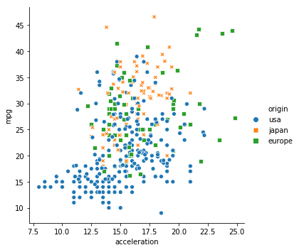
All the contents are from DataCamp